
A Guide on Word Embeddings in NLP💻

I am a Post grad in Bioinformatics . My field of interest and expertise lies mainly in Data Analytics, Machine Learning & Bioinformatics.
Introduction
Natural Language Processing (NLP) is the interdisciplinary field of Computer Science, Artificial Intelligence, and Linguistics, concerned with the ability of computers to understand human language. Word Embeddings is an advancement in NLP that has have skyrocketed the ability of computers to better understand text-based content. It is an approach to represent words and documents in the form of numeric vectors allowing similar words to have similar vector representations. Isn’t making a lot of sense?… Okay, let us start from scratch to develop an understanding of Word Embeddings!
Background
Given a supervised learning task to predict which tweets are about real disasters and which ones are not (classification). Here the independent variable would be the tweets (text) and the target variable would be the binary values (1: Real Disaster, 0: Not real Disaster). Now, Machine Learning and Deep Learning algorithms only take numeric input. So how do we convert tweets to their numeric values? Let’s dive deep.
Bag of Words (BOW)
The bag of words is a type of vectorization technique of text where each value in the vector would represent the count of words of a document/sentence.
Let’s take a small part of disaster tweets, 4 tweets, to understand how BOW works:-
'kind true sadly’,
‘swear jam set world ablaze’,
‘swear true car accident’,
‘car sadly car caught up fire’
To create BOW we use Scikit-learns CountVectorizer, which tokenizes a collection of text documents, builds a vocabulary of known words, and encodes new documents using that vocabulary.
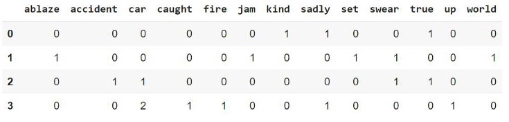
Here the rows represent each document (4 in our case), the columns represent the vocabulary (unique words in all the documents) and the values represent the count of the words of the respective rows. In the same way, we can apply CountVectorizer on the complete training data tweets (11,370 documents) and obtain a matrix that can be used along with the target variable to train a machine learning/deep learning model.
Term Frequency — Inverse Document Frequency (TF-IDF) Let’s see how vectorization is done in TF-IDF -

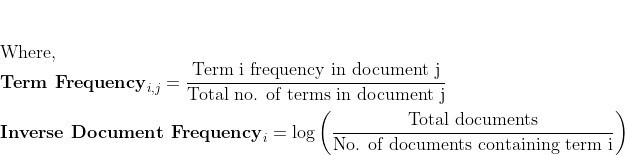
To create TF-IDF vectors, we use Scikit-learns TfidfVectorizer. After applying it to the previous 4 sample tweets, we obtain -
Similar to BOW, the rows represent each document, the columns represent the vocabulary, and the values are tf-idf(i,j) obtained through the above formula. This matrix obtained can be used along with the target variable to train a machine learning/deep learning model.
Challenges:
Now let’s discuss the challenges with the two text vectorization techniques we have discussed till now. In BOW, the size of the vector is equal to the number of elements in the vocabulary. If most of the values in the vector are zero then the bag of words will be a sparse matrix. Sparse representations are harder to model both for computational reasons and also for informational reasons. Also, in BOW there is a lack of meaningful relations and no consideration for the order of words. While the TF-IDF model contains the information on the more important words and the less important ones, it does not solve the challenge of high dimensionality, sparsity and unlike BOW it also makes no use of semantic similarities between words.
Solution: Word Embedding Word Embeddings is a technique where individual words are represented as real-valued vectors in a lower-dimensional space. Representing words as real-valued vectors captures inter-word semantics. Each word is represented by a real-valued vector with tens or hundreds of dimensions. A word vector with 100 values represents 100 unique features.
Let us now discuss two different approaches to getting word embeddings. We’ll also look at the hands-on part!
Word2Vec: Word2Vec method was developed by Google in 2013. The method involves iteration over a corpus of text to learn the association between the words. It relies on a hypothesis that the neighboring words in a text have semantic similarities between each other. It uses cosine similarity metric to measure the semantic similarity. Cosine similarity is equal to Cos(angle) where the angle is measured between the vector representation of two words/documents.
Word2Vec has two neural network-based variants:
- Continuous Bag of Words (CBOW) and
Skip-gram.
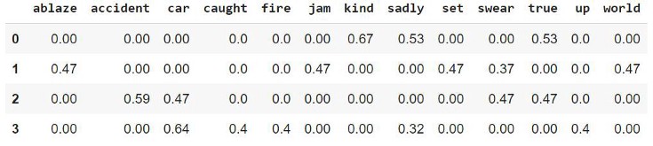
CBOW — Let us understand the concept of context and current word for CBOW.
In CBOW, we define a window size. The middle word is the current word and the surrounding words (past and future words) are the context. CBOW utilizes the context to predict the current words. Each word is encoded using One Hot Encoding in the defined vocabulary and sent to CBOW neural network.
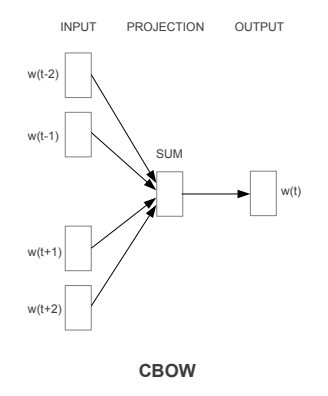
The hidden layer is a standard fully-connected Dense layer. The output layer outputs probabilities for the target word from the vocabulary.
- Skip-gram — Skip-gram is slightly different from CBOW, as it uses the current word to predict the context.
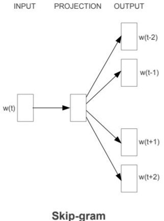
The end goal of Word2Vec (both variants) is to learn the weights of the hidden layer. The hidden weights, we’ll use them as our word embeddings!! Let’s now see the code for creating custom word embeddings using Word2Vec-
Import Libraries:
         from gensim.models import Word2Vec
         import nltk
         import re
         from nltk.corpus import stopwords
Preprocess the Text:
         #Word2Vec inputs a corpus of documents splitted into constituent words
          corpus = []
          for i in range(0,len(X)):
          tweet = re.sub(“[^a-zA-Z]”,” “,X[i])
          tweet = tweet.lower()
          tweet = tweet.split()
          corpus.append(tweet)
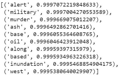
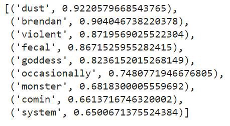
Here is the exciting part! Let’s try to see the most similar words (vector representations) of some random words from the tweets -
model.wv.most_similar(‘disaster’)
Output -
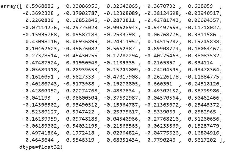
The embedding vector of ‘disaster’ -
GloVe: Global Vector for word representation
GloVe method was developed at Stanford by Pennington, et al. Unlike Word2Vec, which creates word embeddings using local context, GloVe focuses on global context to create word embeddings which gives it an edge over Word2Vec. In GloVe, the semantic relationship between the words is obtained using a co-occurrence matrix.
Consider two sentences -
- I am a data science enthusiast
- I am looking for a data science job
The co-occurrence matrix for involved in GloVe would look like this for the above sentences -
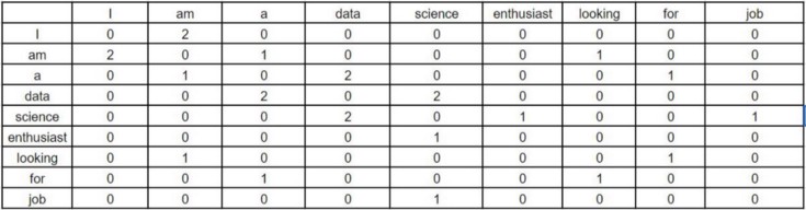
Window Size = 1
Each value in this matrix represents the count of co-occurrence with the corresponding word in row/column. Observe here — this co-occurrence matrix is created using global word co-occurrence count (no. of times the words appeared consecutively; for window size=1). If a text corpus has 1m unique words, the co-occurrence matrix would be 1m x 1m in shape. The core idea behind GloVe is that the word co-occurrence is the most important statistical information available for the model to ‘learn’ the word representation.
Let’s now see an example from Stanford’s GloVe paper of how the co-occurrence probability rations work in GloVe. “For an example, consider the co-occurrence probabilities for target words ice and steam with various probe words from the vocabulary. Here are some actual probabilities from a corpus of 6 billion word:”
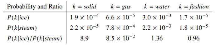
Here,

Let’s take k = solid i.e, words related to ice but unrelated to steam. The expected Pik /Pjk ratio will be large. Similarly, for words k which are related to steam but not to ice, say k = gas, the ratio will be small. For words k like water or fashion, that are either related to both ice and steam or neither to both respectively, the ratio should be approximately one. The probability ratio is able to better distinguish relevant words (solid and gas) from the irrelevant words (fashion and water) than the raw probability. It is also Abe to better discriminate between two relevant words. Hence in GloVe, the starting point for word vector learning is ratios of co-occurrence probabilities rather than the probabilities themselves. To understand the derivation of loss function used in this method:
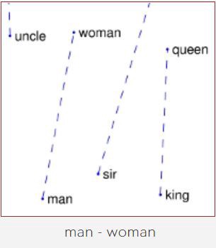 Source: Visualization of GloVe Word Embeddings. King — Man + Woman = Queen
Enough of the theory. Time for the code!
Import Libraries
            import nltk
            import re
            from nltk.corpus import stopwords
            from glove import Corpus, Glove
Text Preprocessing:
         #GloVe inputs a corpus of documents splitted into constituent words
         corpus = []
         for i in range(0,len(X)):
         tweet = re.sub(“[^a-zA-Z]”,” “,X[i])
         tweet = tweet.lower()
         tweet = tweet.split()
         corpus.append(tweet)
Train the word Embeddings:
              corpus = Corpus()
              corpus.fit(text_corpus,window = 5)
              glove = Glove(no_components=100, learning_rate=0.05)
              #no_components = dimensionality of word embeddings = 100
              glove.fit(corpus.matrix, epochs=100, no_threads=4, verbose=True)
              glove.add_dictionary(corpus.dictionary)
Find most similar -
glove.most_similar(“storm”,number=10)
Output -
Conclusion
In this blog, we discussed the two techniques for vectorization in NLP that are Bag of Words and TF-IDF, their drawbacks, and how word-embedding techniques like GloVe and Word2Vec overcome their drawbacks by dimensionality reduction and context similarity.
Word embeddings can be used to train deep learning models like GRU, LSTM, Transformers which have been successful in NLP tasks such as sentiment classification, name entity recognition, speech recognition, etc.
Now you know how word embeddings have benefited your day-to-day life as well.
Happy Learning!!


