A critical phase in machine learning practice is hyperparameter tuning(HP). The performance of ML algorithms’ prediction can be significantly impacted by HP tuning. An ML algorithm’s HPs are often configured through a process of trial and error. It can take a long time to manually select a good set of values, depending on how long the ML algorithm has been trained. As a result, current research in HP for ML algorithms is concentrated on improving HP tuning methods.

Parameters and hyperparameters define machine learning models. The split-feature and split-point of a node in a CART are two examples of parameters that can be learned from data through training. Hyperparameters should be set before training because they cannot be learned from data.

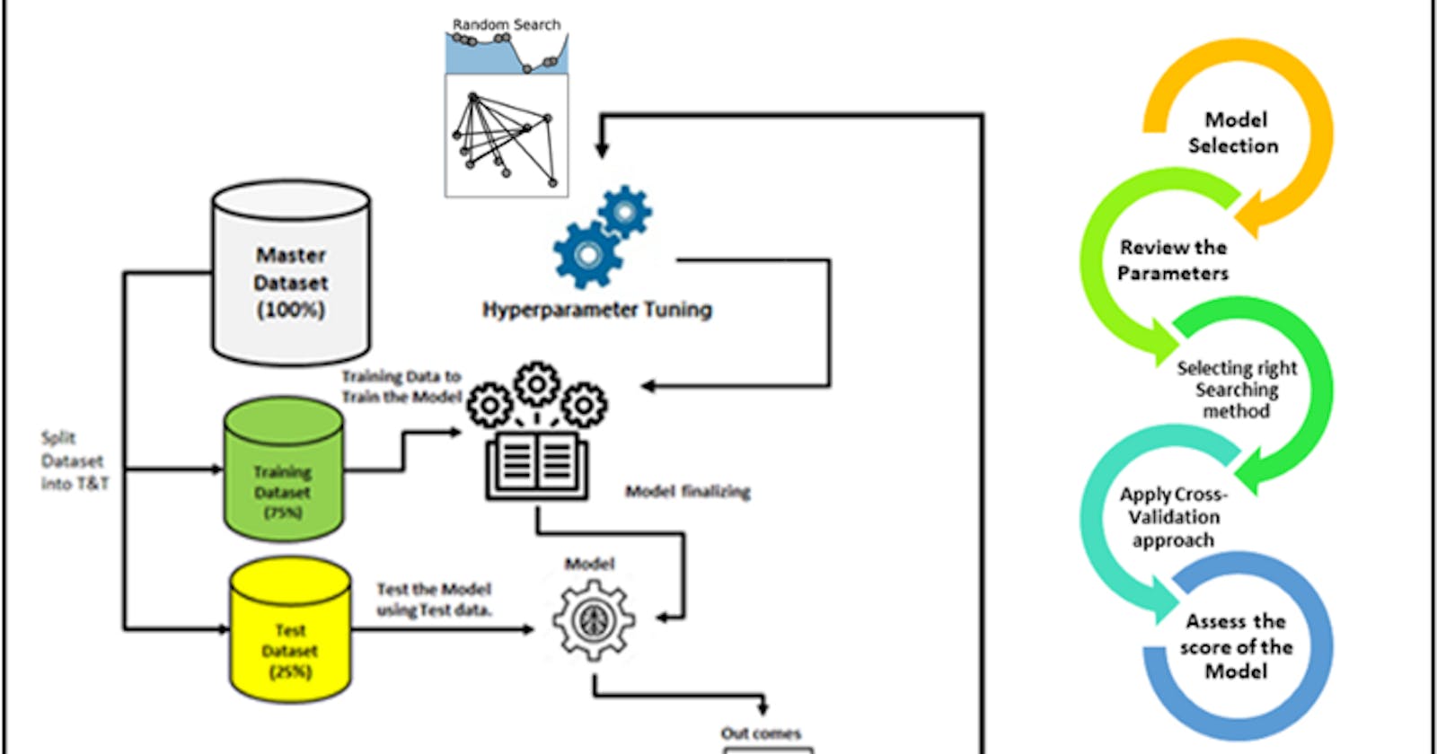
Finding the collection of ideal hyperparameters for the learning algorithm is the process of tuning hyperparameters. In order to solve the problem, one must identify the set of ideal hyperparameters that results in the ideal model. An ideal score is produced by the best model. A model’s predictions and true labels’ agreement are gauged by the score function. For classifiers in Sklearn, the default setting is accuracy, and for regressors, it’s r-squared. Cross-validation is used to assess the generalization capabilities of a model.

High predictive performance for one dataset may not translate to high predictive performance for other datasets, as Hyperparameters values frequently depend on one another (as in the case of SVMs). Therefore, optimizing HPs independently is not a sensible technique because it can take a long time to evaluate just one HP configuration, let alone many. Let’s look at some examples of how to set up hyperparameters tuning for the linear classifier model for a liver patient dataset. The first step is to set up a hyper-parameter grid.

        # Define params_dt
        params_dt = {'max_depth':[2,3,4],'min_samples_leaf':[0.12, 0.14, 0.16, 0.18]}

We will perform a grid search using 5-fold cross-validation to find our decision tree optimal hyperparameters. Note that because grid search is an exhaustive process, it may take a lot of time to train the model.

              # Import GridSearchCV
              from sklearn.model_selection import GridSearchCV
              # Instantiate grid_dt
              grid_dt = GridSearchCV(estimator=dt,
                   param_grid=params_dt,
                   scoring='roc_auc',
                   cv=5,
                   n_jobs=-1)
              #Train the model
               grid_object.fit(X_train, y_train)

We need to evaluate the test set ROC AUC score of grid_dt’s optimal model. In order to do so, we will first determine the probability of obtaining the positive label for each test set observation. You can use the method predict_proba() of an sklearn classifier to compute a 2D array containing the probabilities of the negative and positive class labels respectively along columns.

             # Import roc_auc_score from sklearn.metrics
               from sklearn.metrics import roc_auc_score
                # Extract the best estimator
              best_model = grid_dt.best_estimator_
             # Predict the test set probabilities of the positive class
              y_pred_proba = best_model.predict_proba(X_test)[:,1]
            # Compute test_roc_auc
            test_roc_auc = roc_auc_score(y_test,y_pred_proba)
             # Print test_roc_auc
           print('Test set ROC AUC score: {:.3f}'.format(test_roc_auc))
         Test set ROC AUC score: 0.610

If we compared it to an untuned model classification tree, it would achieve a ROC AUC score of 0.54. So, we achieved a higher ROC score. Similarly, we can try to perform the hyperparameter tuning for a Random-forest. In order to fine-tune RF’s hyperparameters and identify the best regressor, the grid of hyperparameters will be manually set. To achieve this, we will build a grid of hyperparameters and modify the number of estimators, the maximum number of features utilized when splitting each node, and the minimal number of samples (or fraction) per leaf.

                 # Define the dictionary 'params_rf'
                  params_rf = {'n_estimators':[ 100, 350, 500],
                 'max_features':['log2', 'auto', 'sqrt'],
                 'min_samples_leaf':[2, 10, 30]}

After that, we’ll use grid search with three-fold cross-validation to identify rf’s ideal hyperparameters. You’ll use the negative mean squared error measure to rate each model in the grid.

             # Import GridSearchCV
             from sklearn.model_selection import GridSearchCV
            # Instantiate grid_rf
             grid_rf = GridSearchCV(estimator=rf,
                   param_grid=params_rf,
                   scoring='neg_mean_squared_error',
                   cv=3,
                   verbose=1,
                   n_jobs=-1)

Next, we need to evaluate the test set RMSE of grid_rf's optimal model.

      # Import mean_squared_error from sklearn.metrics as MSE 
      from sklearn.metrics import mean_squared_error as MSE
      # Extract the best estimator
       best_model = grid_rf.best_estimator_
       # Predict test set labels
        y_pred = best_model.predict(X_test)
        # Compute rmse_test
        rmse_test = MSE(y_test,y_pred)**(1/2)
        # Print rmse_test
         print('Test RMSE of best model: {:.3f}'.format(rmse_test))
         Test RMSE of best model: 50.558

Thus, we saw from our examples, how we can use Grid search with cross-validation to perform hyperparameter tuning for Random Forest and Decision tree classifiers.